Interpolation for Lagrangian Elements - II

Continuing from where we left off in the previous post, I will explain how I went about finishing tasks #4 to #6 in the list. Just to recall, in the previous blog post, I explained how to create the source finite element space and the FEFunction. I also covered on how to create the target mesh. To interpolate the old FEFunction onto the new mesh, we need to evaluate the old FEFunction on the cell dofs of the new mesh. This can be done using the drivers that I discussed in the first blog post. Here’s how it went…

Task #4 and #5

Let us say, we have a Lagrange FESpace defined on model₂ called V₂.

order = 2
reffe = ReferenceFE(lagrangian, Float64, order)
V₂ = FESpace(model₂, reffe) # Recall: model₂ = CartesianDiscreteModel(domain,partition; map=rndm)

Now we evaluate the function old function fh on the new mesh. One way to do this could be:

phys_point = get_cell_points(get_fe_dof_basis(V₂)).cell_phys_point
fₕ_phys_coords(x) = evaluate(fₕ, x)
phys_point_fx = lazy_map(fₕ_phys_coords, phys_point)
gₕ = CellField(V₂, phys_point_fx)

The first line creates a LazyArray named phys_point which consists of coordinates of the new mesh in the physical space of V₂ (Note that the reference domain is the same for V₁ and V₂). Then in the third line, we create a LazyArray of function values of fh evaluated at phys_point using the map x -> evaluate(fₕ,x), defined in the second line. This works, because evaluate(fₕ,x) now works for arbitrary points (see this post here). Thus, the variable phys_point_fx represents a cell-wise LazyArray consisting of the function value fₕ evaluated on the physical points of V₂. Using phys_point_fx, we build a CellField object on the finite element space V₂.

Now gₕ is the interpolated function we are looking for in V₂. Now, the previous paragraph describing the procedure maybe a little unclear with all the technical terms, but it can be realized quite easily by simply running the line one-by-one in the REPL. Also, this method should work for FESpace of different orders, for example, from order=2 in the old mesh to say, order=1 in the new mesh. Try it out!

Task #6

The last task is to check the result of the code. The first way is by the good old visual inspection:

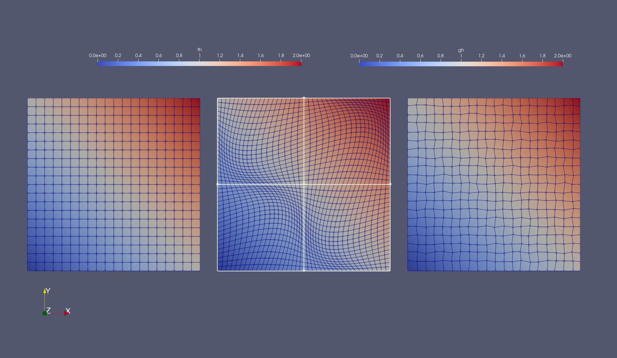Seems cool enough! But we want to know for sure. So, we try to build a simple test for random points as follows

using Test

@testset begin
    xs = [VectorValue(rand(2)) for i ∈ 1:10]
    for x in xs
        @test isapprox(evaluate(gₕ,x), evaluate(f,x), atol=1e-7)
    end
end

We begin by first creating an array xs using one of the coolest features of Julia - Array Comprehension. Then we loop over the elements of xs and check whether the new function gₕ evaluates to the same value of the infinite dimensional function f(x) up to a tolerance. I declared f(x) = x[1] + x[2] and interpolated to a second order FESpace, which means gh should give a good approximation of the function at arbitrary points in the domain. Depending on your mesh, It should throw out something like this

Test Summary: | Pass  Total
test set      |   10     10

In fact, it should be exact provided everything is good. And with this now, we come to the challenges associated with implementing this algorithm.

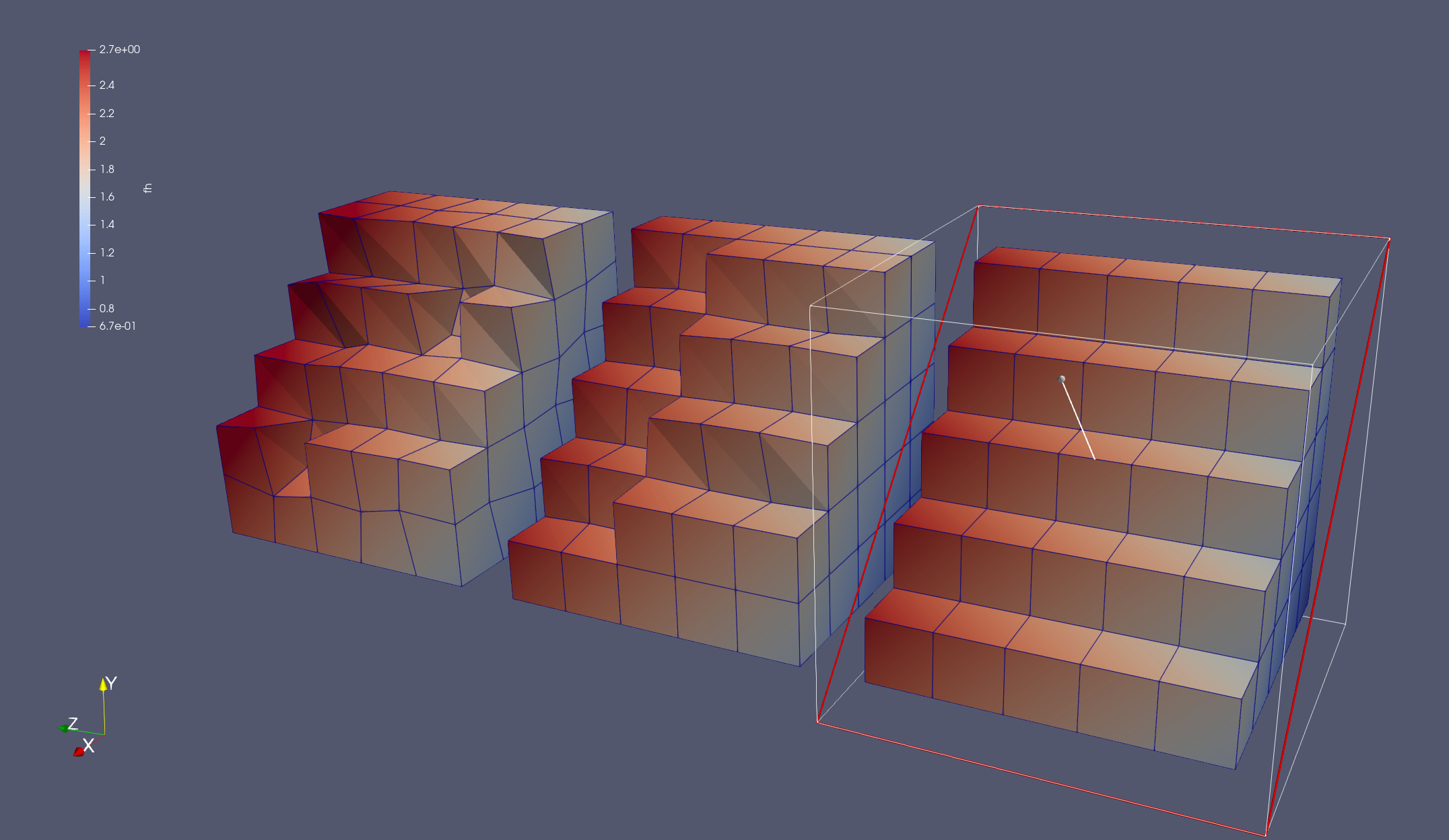
• Distorted Elements: For highly distorted elements, like the second one in the image above, the inverse map from physical space to reference space becomes difficult to compute. This is common in finite elements and hence such distorted elements are avoided. In order to get good approximations, one needs to compute the inverse maps accurately. This can be done by specifying a more robust non-linear solver to build the inverse map. I will cover this issue in detail in a separate blog entry soon.

• What about other elements? I am working on it as we speak. This is one of the objectives of my GSoC project and I hope to have a solution soon! Until then, check out the task list here.

For the more enthusiastic readers, I wrote a full set of test cases that works for n-dimensions on both sinusoidal and random meshes. Click on the image below to take you there. I will keep you updated on my progress, as now we move into the mid-term evaluations. I should have one more post before then. See you guys in the next one!