Interpolation for Lagrangian Elements - I

It’s time for another GSoC project update. During the last couple of weeks, I have been working on building the method for performing interpolations between different meshes. I will be explaining this task list in detail and finish up by describing where this will eventually lead to. I will also briefly talk about some of the challenges I faced as I was going through the list. There are six tasks in the list, and I have listed them down below:

• Build a cartesian mesh along with the FE Space etc.
• Interpolate and exact solution in the FE Space.
• Create a new mesh using the old mesh. Use the map option to perturb the original mesh. Example meshes here in Fig 6.1.
• Evaluate the old function in the new node positions.
• Create an FEFunction struct using the nodal values in the previous step.
• Check the result of the new FEFunction.

Two things before we start. I am maintaining another repository containing some of the code I use to test my ideas. To explain the tasks in the list, I will be considering this code here:

• GSoC-2021/Interpolation/interpolate.jl

Also, I have split this topic into two blog posts to better explain the tasks individually. I will be discussing the first three tasks in this post. For the other three tasks, head on here. Here we go!

Task #1

The first step is to build a cartesian mesh along with the finite element space. This is a simple process which can be done by running

# Build the cartesian model
domain = (0,1,0,1)
partition = (10,10)
model = CartesianDiscreteModel(domain, partition)

to build the model and running

# Build a second order reference finite element space
reffe = ReferenceFE(lagrangian, Float64, 2)

# Next build an FESpace on the mesh using the reference finite element
V₁ = FESpace(model, reffe)
Ω₁ = Triangulation(model)

to construct the finite element space. This FESpace contains second order Lagrangian finite elements. I will be using this space as the source, where I will be interpolating FEFunction defined on this space to other Lagrangian FESpaces. Simple enough!

Task #2

The next step is to interpolate an exact solution onto the new FESpace. This is done by using the interpolate_everywhere method available in Gridap.

# An exact solution
f(x) = x[1] + x[2]
# A finite element (discrete) function defined on V₁.
fₕ = interpolate_everywhere(f, V₁)

Now, fₕ is a finite element function defined cell-wise inside V₁. So now, running for example

julia> get_cell_coordinates(Ω₁)

20×20 LazyArray{FillArrays.Fill{Broadcasting{Reindex{Gridap.Geometry.CartesianCoordinates{2, Float64, typeof(identity)}}}, 2, Tuple{Base.OneTo{Int64}, Base.OneTo{Int64}}}, Vector{VectorValue{2, Float64}}, 2, Tuple{Gridap.Geometry.CartesianCellNodes{2}}}:
 [(0.0, 0.0), (0.05, 0.0), (0.0, 0.05), (0.05, 0.05)] ⋯
 ⋮

julia> get_cell_dof_values(fₕ)

400-element LazyArray{FillArrays.Fill{Broadcasting{PosNegReindex{Vector{Float64}, Vector{Float64}}}, 1, Tuple{Base.OneTo{Int64}}}, Vector{Float64}, 1, Tuple{Table{Int32, Vector{Int32}, Vector{Int32}}}}:
 [0.0, 0.05, 0.05, 0.1]
 ⋮

The second command generates a LazyArray containing the cell-wise degree of freedom values of fₕ, which in case of Lagrangian Elements is simply the point-value of functions. This can differ in case of other elements, for example, the Raviart-Thomas elements which will be considered later.

So far so good … Now we have built the associated Source problem. The next step is to define the target mesh and finite element space.

Task #3

The target mesh in reality could be anything. But for our example here, Gridap offers a way to create different meshes by providing an option map to specify a function that maps the Cartesian points to the new mesh points.

partition = (40,40)
model₂ = CartesianDiscreteModel(domain,partition; map=sinusoidal_map)

The function sinusoidal_map defines the map that defines the position of the new mesh points. I considered two different maps,

• A sinusoidal map.
• A random perturbation.

The function sinusoidal_map for the sinusoidal mapping defined below

function sinusoidal_map(p::Point)
    r, s = p
    x = r + 0.08*sin(2π*r)*sin(2π*s)
    y = s + 0.08*sin(2π*r)*sin(2π*s)
    Point(x,y)
end

The function takes the point p from the old mesh, applies the mapping and returns the new point. The map is taken from Figure 6.1 in this paper here.

The random map is much cooler and is considered in the script here. Do take a look!

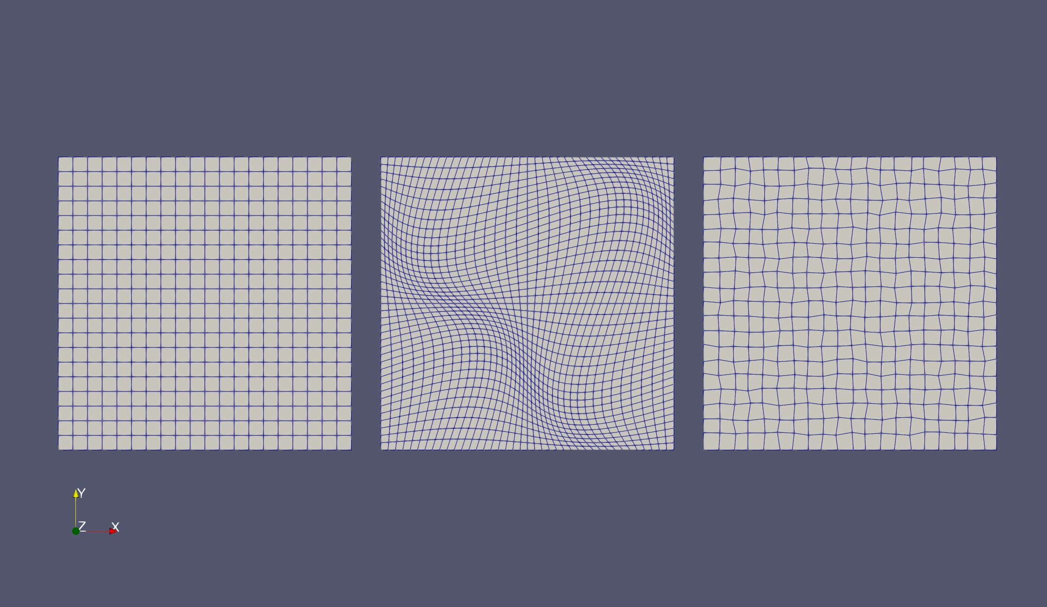
The three meshes are shown in the Figure below. The leftmost image is the source, the middle is the sinusoidal mesh and the rightmost image is the randomly perturbed mesh.

Now we are set to perform the interpolation. See my next blog post for Tasks #4 to #6.