Multiscale Methods

We are interested in developing efficient numerical methods to solve partial differential equations with highly oscillatory data. For example, we look at the wave equation model problem

\[\begin{align} &\partial_t^2 u(x,t) - \nabla \cdot \left(A_{\varepsilon}(x) \nabla u(x,t)\right) = f(x,t), \quad (x,t) \in \Omega \times (0,T],\\ &u(x,0) = u_0(x), \quad x \in \Omega,\\ &u = 0, \quad (x,t) \in \partial \Omega \times (0,T]. \end{align}\]

The diffusion coefficient \(A_{\varepsilon}(x)\) oscillates at a fine scale \(\varepsilon \ll 1\). Traditional finite element methods require the mesh size \(h\) to resolve the underlying oscillation scale in order to obtain reasonably accurate approximations of the solution. We are interested in developing higher-order multiscale methods that yields a discrete linear system on a coarse mesh (of size \(H \gg h\)) by constructing spaces with enhanced approximation properties. These bases also have a compact support on the domain, potentially resulting in a sparse linear system that is computationally tractable and high-order accurate. A brief description of our work so far.

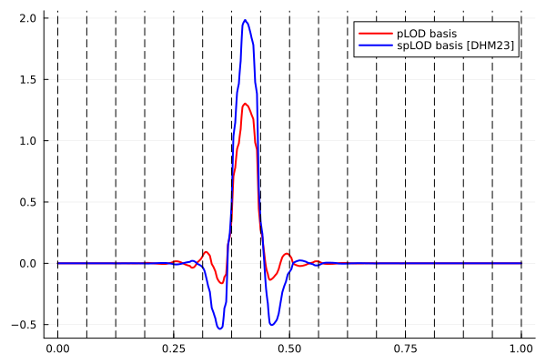
The canonical high-order multiscale bases discussed in (shown in the left panel of the figure below)

[DHM23] Dong, Z., Hauck, M., & Maier, R. (2023). An improved high-order method for elliptic multiscale problems. SIAM Journal on Numerical Analysis, 61(4), 1918-1937.

Maier, R. (2021). A high-order approach to elliptic multiscale problems with general unstructured coefficients. SIAM Journal on Numerical Analysis, 59(2), 1067-1089.

yields suboptimal convergence rates when applied to time dependent PDEs.

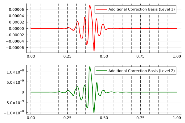
In my postdoc at Umeå University, we looked at improving the method by defining suitable additional correction bases (shown in the middle panel below) on the coarse scale. These bases are then used to expand a time-dependent correction term added to the original multiscale solution in order to improve the overall error. We discuss the construction of the bases and prove optimal convergence rates in our papers:

Kalyanaraman, B., Krumbiegel, F., Maier, R., & Wang, S. (2026). Enriched higher-order multiscale approaches with applications to wave propagation. Submitted arXiv [Math.NA]. Retrieved from https://arxiv.org/abs/2605.30118

Kalyanaraman, B., Krumbiegel, F., Maier, R., & Wang, S. (2025). Optimal higher-order convergence rates for parabolic multiscale problems. Submitted arXiv [Math.NA]. Retrieved from https://arxiv.org/abs/2510.09514

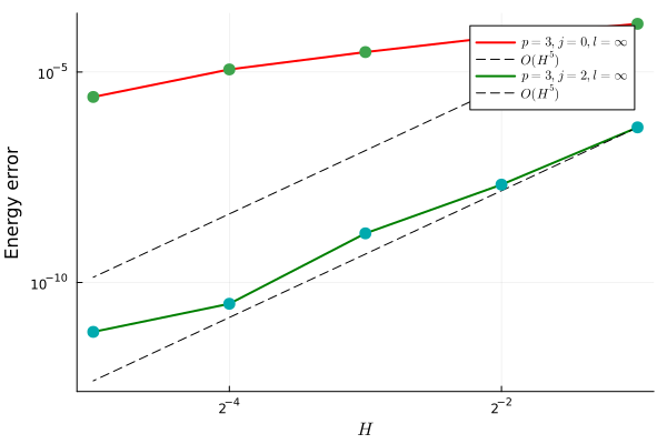
As shown in the right panel below, we observe that the convergence rates are optimal after employing the additional correction terms.

Multiscale basis functions	Additional correction basis	Convergence rates for the wave equation

Ice Shelf Vibrations

Consider an ice-shelf which is assumed to be a two dimensional elastic body. The ice-shelf is fixed at the landward end \(x=L\) (right) and free to vibrate at the seaward end \(x=0\) (left). Open ocean of depth \(H\) exists for \(x<0\) and a cavity region filled with water exists underneath the ice-shelf \(0<x<L\). The fluid flow is governed by the potential flow theory and the vibration of the ice-shelf is governed by linear-elasticity theory.

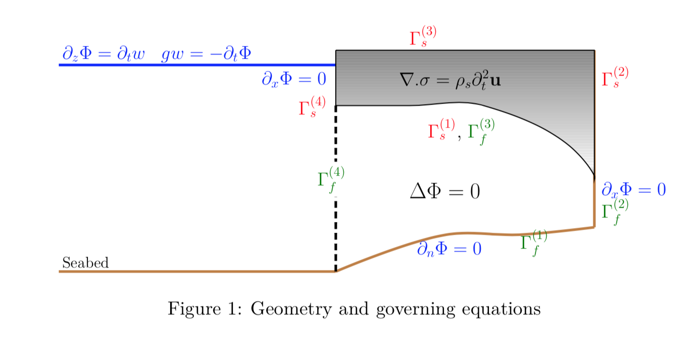
The objective of the problem is to study the vibrations of the ice-shelf in response to the waves generated in the open ocean region. The problem is solved using the finite element method and the displacement of the ice-shelf are shown in the videos below. The code is available on Github which was also published in the Journal of Open Source Software. The video below compares the vibration of an ice-shelf (modelled as a clamped elastic body) vs an iceberg (modelled as a free elastic body) subject to the same incident wave forcing. The semi-infinite boundary in Figure 1 is treated using a non-local boundary condition defined on the boundary \(\Gamma_f^{(4)}\). See the abstract of the presentation in 34th International Workshop on Water Waves and Floating Bodies and also my paper

Kalyanaraman, B., Meylan, M. H., Bennetts, L. G., & Lamichhane, B. P. (2020). A coupled fluid-elasticity model for the wave forcing of an ice-shelf. Journal of Fluids and Structures, 97, 103074.

Gradient Recovery for Virtual Element Methods

Gradient recovery methods are popular numerical techniques to approximate the gradient of the solution. They have super convergence property and are used in adaptive refinement. Gradient recovery techniques based on oblique projection are well studied for the finite element methods.

A gradient recovery technique based on the oblique projection can be defined for virtual element methods on Polygonal meshes. In the virtual element setting, the gradient recovery operator projects \(\nabla u_h\) by finding \(g_h^k = \text{Q}_h\left(\frac{\partial u_h}{\partial x_k}\right) \in V_h\) for \(k=1,2\) such that

\[\begin{equation} \sum_{K}\left(\Pi_K^{0}g_h^k, \Pi_K^{0} \mu_j\right)_K = \sum_{K}\left(\frac{\partial (\Pi_K^{0} u_h)}{\partial x_k}, \Pi_K^{0}\mu_j\right)_K. \end{equation}\]

with \((x_1,x_2) = (x,y)\) and the functions \(\mu_j \in \mathcal{M}_h := \text{span}\{\mu_1,\mu_2,\cdots,\mu_N\}\) satisfy the bi-orthogonal relation

\[\begin{equation} \left(\Pi^{0}_K \varphi_i, \Pi^{0}_K \mu_j\right)_K = c_j \delta_{ij} \quad \forall K \in \mathcal{T}_h.\label{eq:biorth} \end{equation}\]

where the scaling factors \(c_j\) are obtained using mass lumping. We can observe higher rates of convergence for the gradient which is shown in the Figure below.

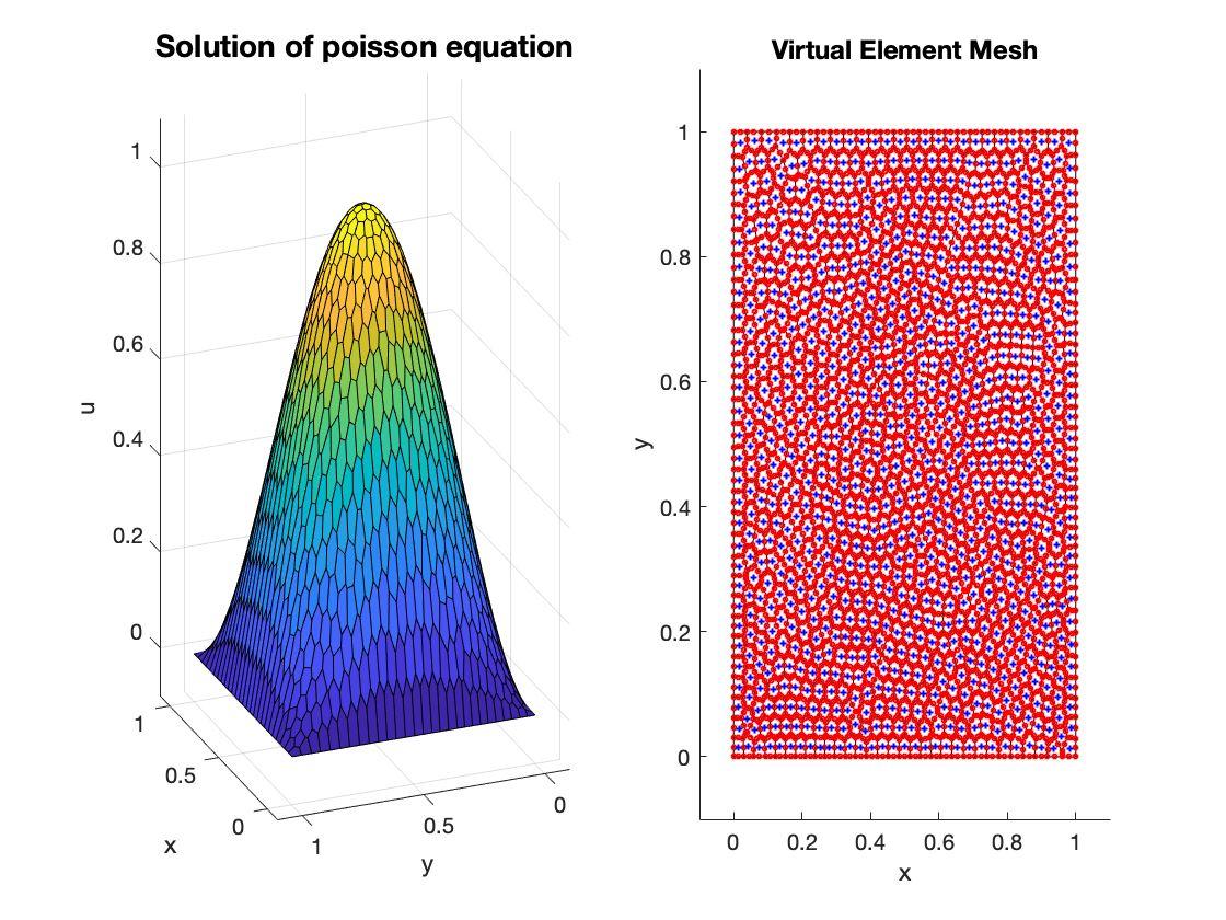
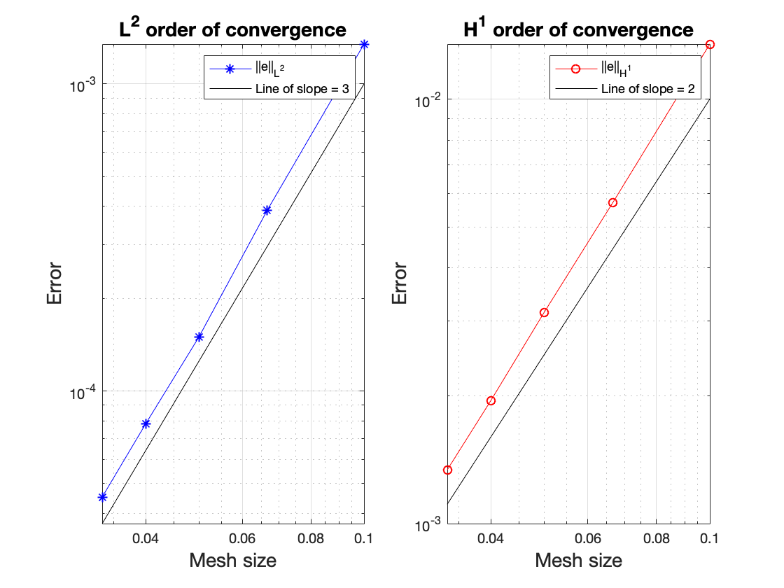
You can find the full article online published in the ANZIAM Journal. Do read my blog post on how it can be made better!! Also, check out this repository for the MATLAB codes.